What Are Multimodal Embeddings? How AI Understands Text, Images, Audio & More

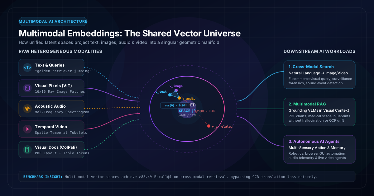
1. The Sensory Blind Spot: When Text-Only AI Meets Physical Reality

Imagine an emergency in an industrial power plant at 2:15 AM. A gas turbine generator triggers a critical vibration alarm. The senior reliability engineer uploads three raw files into the facility’s enterprise AI diagnostic assistant:

1. A 5-second acoustic WAV recording captured by a microphone mounted on the high-pressure compressor housing.
2. A high-resolution ultrasonic B-scan cross-section image showing an internal structural anomaly deep within rotor blade #14.
3. A 140-page PDF OEM maintenance manual containing complex hydraulic flow schematics, wiring diagrams, and clearance tolerance tables.

The engineer types a single urgent query into the terminal:

"Analyze the attached acoustic whine and ultrasonic slice. Have we observed this exact rotor resonance harmonic and subsurface micro-delamination before? Retrieve matching historical repair logs, identify the root failure mode, and cite the maximum allowable runout tolerance from Section 8 of the manual."

If the organization's system relies on a traditional text-only Retrieval-Augmented Generation (RAG) pipeline—the kind powering 90% of enterprise AI deployments built between 2023 and 2025—the pipeline collapses into a catastrophic sequence of failures:

The system queries its vector database using a text embedding model (such as text-embedding-3-large). Because the text embeddings were generated from empty transcripts and vague captions, the database returns irrelevant historical incidents about fuel valve calibrations.

The AI did not fail because its reasoning engine lacked intelligence. It failed because text is an extreme low-bandwidth compression of physical reality. Forcing all sensory perception—acoustics, visual textures, spatial layouts, and video motion—through a narrow bottleneck of natural language tokens is called Semantic Transcoding Loss.

To solve this fundamental flaw, modern AI engineering had to abandon the text-only paradigm and build something far more profound: Multimodal Embeddings.

2. What Are Multimodal Embeddings? Mathematical & Geometric Intuition

At its core, an embedding is a translation mechanism. It maps an unstructured, qualitative piece of human experience into a dense mathematical vector—an ordered array of floating-point numbers in a continuous vector space:

In a classical unimodal setup, text has its own vector space \(\mathcal{S}_{\text{text}}\), while images reside in \(\mathcal{S}_{\text{image}}\). If you compute the dot product between a vector produced by a text embedder and a vector produced by an image embedder, the result is mathematical nonsense—equivalent to multiplying temperature by velocity. They operate in completely unrelated coordinate systems with zero shared geometry.

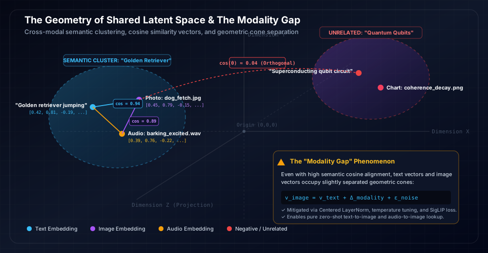
Multimodal embeddings eliminate this barrier by establishing a Shared Latent Manifold (Joint Embedding Space).

In this shared space, semantic concepts exist independently of how they are sensed. If you embed:

• The text string: "A golden retriever leaping into a lake to catch a red ball"
• A 4K photograph of that exact golden retriever mid-air over the water
• A 3-second audio recording of water splashing accompanied by an excited canine bark
• A 10-second video clip capturing the entire sequence in motion

The multimodal embedding model maps all four disparate sensory streams to virtually identical coordinates in \(\mathbb{R}^d\). Their geometric distance is minimal, and their cosine similarity approaches 1.0:

Conversely, an unrelated concept—such as a PDF page describing a semiconductor patent or the sound of an espresso machine—maps to an orthogonal coordinate in the hypersphere, yielding a cosine similarity near \(0.0\).

3. Converting Sensory Data to Numbers: How Each Modality Is Encoded

How can a neural network take raw audio air pressure, a grid of colored pixels, and an alphanumeric sentence, and translate them all into vectors that speak the same mathematical dialect?

Each sensory modality requires a dedicated transformation pipeline before reaching the shared manifold:

A. Text Encoding (Byte-Pair Tokens → Transformers)

Text is discrete and sequential. The transformation process follows four key steps:

1. Tokenization: The sentence is split into subword units using Byte-Pair Encoding (BPE) or WordPiece (e.g., "retriever" → ["re", "trie", "ver"]).
2. Vocabulary Lookup & Positional Embedding: Each token ID is converted into an initial embedding vector, and sinusoidal or learned positional encodings are added to preserve grammatical syntax.
3. Self-Attention Layers: A transformer encoder (such as RoBERTa or a causal transformer like GPT/LLaMA) computes multi-head self-attention, allowing every word to contextualize its meaning based on surrounding words.
4. Pooling & Projection: The final hidden states are pooled (either by taking the [CLS] token or via mean pooling across all tokens) and passed through a learned linear projection layer \(W_{\text{text}}\) to match the target shared dimension \(d\).

B. Image Encoding (Pixels → Vision Transformers)

Unlike text, images are continuous, two-dimensional spatial arrays of RGB pixels (e.g., \(3 \times 224 \times 224\)). Modern architectures rely on the Vision Transformer (ViT):

1. Patch Extraction: The image is cut into a non-overlapping grid of patches, typically \(16 \times 16\) pixels. An image of resolution \(224 \times 224\) yields \(14 \times 14 = 196\) distinct visual patches.
2. Linear Patch Projection: Each \(16 \times 16 \times 3 = 768\)-dimensional patch is flattened and linearly projected into a vector of dimension \(D_{\text{model}}\).
3. Spatial Positional Encodings: Because transformers are permutation-invariant, 2D positional embeddings are added to each patch vector so the model knows which patch is in the top-left corner versus bottom-right.
4. Self-Attention & Visual Pooling: The patch vectors pass through transformer blocks where attention heads learn visual relationships (textures, edges, object shapes, backgrounds). An attention-pooling head or [CLS] token outputs a single global image vector \(\vec{v}_{\text{image}}\).

C. Audio Encoding (Acoustic Waves → Mel-Spectrograms)

Audio is recorded as a one-dimensional pressure waveform fluctuating over time (e.g., 44,100 samples per second). Deep learning models rarely process raw waveforms directly. Instead, they transform sound into an image of sound:

1. Short-Time Fourier Transform (STFT): The audio signal is windowed into short overlapping segments (e.g., 25ms), and a Fast Fourier Transform is applied to decompose the wave into its constituent frequencies.
2. Log-Mel Filterbank: The linear frequencies are mapped onto the nonlinear Mel scale, which mimics how the human cochlea perceives pitch (higher resolution at low frequencies, wider bins at high frequencies). The result is a 2D Log-Mel Spectrogram where the X-axis is time, the Y-axis is frequency, and the pixel intensity is energy/amplitude.
3. Audio Spectrogram Transformer (AST): The 2D spectrogram is treated exactly like an image! It is divided into time-frequency patches (e.g., \(16 \times 16\)), equipped with temporal and frequency positional embeddings, and processed by a standard Vision Transformer.
4. Projection: The final output is pooled into an acoustic embedding vector \(\vec{v}_{\text{audio}} \in \mathbb{R}^d\).

D. Video Encoding (Spatio-Temporal Dynamics)

Video adds the critical dimension of time to visual data. Processing video frame-by-frame ignores motion, velocity, and cause-and-effect:

• 3D Spatio-Temporal Tubelets: Video models (such as ViViT or VideoMAE) extract 3D "tubelet" tokens of size \(16 \times 16 \times 2\) (16x16 spatial pixels across 2 consecutive frames).
• Factorized Temporal Attention: To avoid quadratic complexity explodes, models split attention: first spatial self-attention within each frame, followed by temporal attention across time frames.
• Motion Vector Fusion: Optical flow and audio soundtrack tracks are fused into the final temporal representation, capturing actions like "opening a bottle" versus "closing a bottle".

E. Visual Document Encoding (ColPali & Late Interaction)

Enterprise PDFs, financial reports, and blueprints contain a hybrid mix of text, typography, layout, borders, and charts. Traditional OCR scrambles this structure.

Pioneered by ColPali (built on top of PaliGemma), modern systems render the entire document page as a high-resolution image. The vision encoder breaks the page into visual patch tokens, generating a multi-vector representation where every patch preserves the visual font size, bold headers, table cells, and graphical lines without ever running OCR.

4. Architectural Blueprints: How Models Connect the Modalities

How do we train disparate encoders so that their outputs land in the exact same coordinate space? Modern AI architectures employ four distinct training paradigms:

A. Dual Encoders & Contrastive Learning (CLIP & SigLIP)

Pioneered by OpenAI's CLIP (Contrastive Language-Image Pre-training) in 2021 and perfected by Google's SigLIP, the Dual Encoder architecture uses two separate towers: an Image Tower \(f_{\text{img}}\) and a Text Tower \(f_{\text{text}}\).

The model is trained on hundreds of millions of (image, text) pairs \((I_i, T_i)\). During each training step with batch size \(N\):

• There are \(N\) correct diagonal pairs (positive examples).
• There are \(N^2 - N\) incorrect off-diagonal combinations (negative examples).

CLIP trains both encoders simultaneously using the InfoNCE symmetric cross-entropy loss:

The loss pulls matching (image, text) vectors together while aggressively repelling all non-matching pairs.

B. Universal Modality Binding (Meta ImageBind)

What if you want to connect text, images, audio, depth maps, thermal infrared scans, and IMU inertial motion sensors? Collecting millions of paired (Thermal, Audio) or (Depth, IMU) datasets is practically impossible.

Meta solved this with ImageBind in 2023. ImageBind observed that images are naturally paired with almost all other modalities:

• Web video naturally binds Video + Audio.
• Smartphones and lidar cameras naturally bind Images + Depth.
• Thermal sensors naturally capture Thermal + RGB Video.
• Wearables record Video + IMU Motion Sensors.

By using Image as the binding hub, ImageBind aligns every other modality to the image representation space. Because Modality A is aligned with Image, and Modality B is aligned with Image, Modality A and B automatically become aligned with each other without a single direct training pair!

This unlocks zero-shot cross-modal retrieval: you can search an audio database using a thermal camera frame, or query a video library using an IMU motion curve.

C. Late Interaction Multi-Vector Encoders (ColPali)

Dual encoders like CLIP suffer from a major limitation known as the Information Bottleneck: they compress an entire image or document page containing thousands of data points into a single 768-dimensional float array.

Inspired by ColBERT in text search, ColPali avoids single-vector pooling. Instead:

1. The query sentence is embedded into an array of token vectors: \(Q = [\vec{q}_1, \vec{q}_2, \dots, \vec{q}_m]\).
2. The document page image is embedded into an array of patch vectors: \(D = [\vec{d}_1, \vec{d}_2, \dots, \vec{d}_n]\) (typically 1,024 vectors per page).
3. At query time, the system computes the MaxSim (Maximum Similarity) score:

For every single query word, MaxSim finds the single visual patch on the page that matches it most closely. If the query asks for "gross margin 2025", the word "margin" snaps directly to the visual table header, while "2025" snaps to the corresponding column cell. This delivers unprecedented retrieval accuracy on visual documents without requiring any OCR.

5. Vector Databases & Production Indexing for Multimodal Data

Generating multimodal embeddings is only half the battle. In a production enterprise system with 50 million images, 10 million audio clips, and 20 million PDF pages, searching for the nearest vector using brute-force dot product would take seconds—an unacceptable latency for real-time systems.

Production systems rely on specialized Vector Databases (such as Qdrant, Milvus, pgvector, and Pinecone) equipped with Approximate Nearest Neighbor (ANN) index algorithms:

HNSW vs. IVF-PQ Indexing

• HNSW (Hierarchical Navigable Small World): Constructs a multi-layer graph where upper layers feature long-range sparse connections and lower layers feature dense local connections. It delivers 98%+ recall with sub-10 millisecond query latency, though it requires keeping the graph in RAM.
• IVF-PQ (Inverted File with Product Quantization): Divides the vector space into Voronoi clusters (IVF) and compresses 1024-dimensional floating-point vectors into short 64-byte quantized codes (PQ). This slashes RAM requirements by 85% to 92%, allowing billions of multimodal embeddings to be indexed cost-effectively on SSDs.

Matryoshka Representation Learning (MRL)

One of the most powerful recent breakthroughs is Matryoshka Embeddings (supported in models like Nomic Embed Vision and OpenAI text-embedding-3).

Named after Russian nesting dolls, MRL forces the neural network to pack the most critical semantic information into the first few dimensions. A model trained with 1024 dimensions can have its vectors sliced down to 256 or 128 dimensions simply by truncating the array:

Named Vector Spaces (Multi-Vector Storage)

In modern databases like Qdrant, a single database record can hold multiple vector representations under different names. For example, a product catalog entry for a running shoe can store:

• visual_vector: 768d vector extracted from the shoe photograph via SigLIP.
• description_vector: 1536d vector extracted from product specs and customer reviews.
• audio_vector: 512d vector extracted from the commercial video soundtrack.

At query time, the system can execute weighted multi-vector search, finding items that match the user's text query while simultaneously respecting visual color filters.

6. Multimodal RAG: Grounding Foundation Models in Visual Reality

Retrieval-Augmented Generation (RAG) is the foundational architecture for enterprise AI. However, the industry is undergoing a massive generational shift from text-only RAG to True Multimodal RAG.

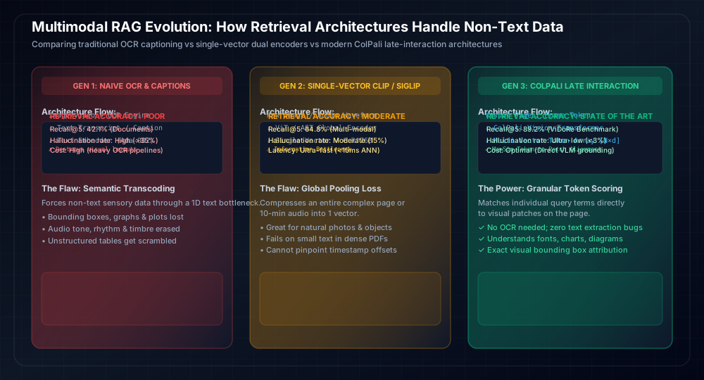
In a modern Multimodal RAG workflow:

1. Cross-Modal Ingestion: Documents are converted into rendered visual pages. Videos are split at scene-cut boundaries into keyframe thumbnails and synchronized audio snippets.
2. Vector Indexing: The visual and acoustic assets are embedded into the shared vector database alongside their metadata payloads (timestamps, bounding box coordinates, page numbers).
3. Retrieval: The user's query (which can be a text string, an image, or a voice prompt) is embedded and used to retrieve the Top-K most relevant visual crops and audio segments.
4. Grounded VLM Synthesis: The retrieved high-resolution image crops and raw transcripts are passed directly into the prompt context of a frontier Vision-Language Model (such as Gemini 2.5 Pro, Claude 3.7 Sonnet, or GPT-4o).
5. Hallucination-Free Reasoning: The VLM does not need to guess what was on the page—it inspects the exact original pixels, citing visual bounding boxes and exact timestamps in its response.

7. Real-World Enterprise Applications

Multimodal embeddings are powering transformative breakthroughs across every major industry:

8. Technical Challenges & The "Modality Gap"

While multimodal embeddings are remarkably capable, production deployments encounter critical engineering bottlenecks:

The Modality Gap Phenomenon

In 2022, researchers at Stanford uncovered a surprising geometric reality: in virtually all contrastively trained multimodal models (including CLIP and OpenCLIP), image embeddings and text embeddings occupy completely disjoint geometric cones within the shared vector space.

Even when an image and a text caption represent the identical concept, their vector representations are separated by a constant modality offset vector:

Why does this happen?

• Initialization Asymmetry: Text and vision encoders are initialized differently, and gradient updates during contrastive learning preserve an initial offset.
• Contrastive Temperature & Narrow Cones: Contrastive loss only requires the correct image to be closer to its paired caption than to negative captions; it does not require them to be identical vectors.
• Dimensionality Imbalance: Text is sparse and discrete, whereas images are continuous and dense with background noise.

Computational & Latency Bottlenecks

Embedding 1,000 text queries takes less than 50 milliseconds on a standard CPU. In contrast, running a high-resolution Vision Transformer (ViT-L/14) on 1,000 high-res images requires significant GPU compute (V100/A100), consuming 15x to 40x more memory bandwidth. Ingesting millions of PDF pages or video streams requires robust asynchronous job queues (such as Ray or Celery) with GPU batching.

9. Evaluation & Benchmarking: How to Measure Quality

How do you evaluate whether a multimodal embedding model is production-ready? Relying on qualitative eyeballing leads to silent production degradation. The AI community uses standard quantitative benchmarks:

10. Production Roadmap: Building a Multimodal Search Pipeline in Python

Let's put theory into practice. Below is a complete, production-grade Python implementation demonstrating how to:

1. Load a modern state-of-the-art multimodal model (OpenCLIP with SigLIP architecture).
2. Initialize an in-memory Qdrant vector database with named vector spaces.
3. Embed both raw images and text queries into the shared coordinate space.
4. Execute a zero-shot cross-modal similarity search (Text Query → Image Retrieval).
5. Pass the retrieved visual evidence to a multimodal LLM for grounded reasoning.

# Install dependencies: pip install torch open_clip_torch qdrant-client pillow
import torch
import open_clip
from PIL import Image
from qdrant_client import QdrantClient
from qdrant_client.models import Distance, VectorParams, PointStruct

# 1. Initialize Device and Load Modern SigLIP Multimodal Model
device = "cuda" if torch.cuda.is_available() else "cpu"
print(f"Active compute hardware: {device}")

# We use ViT-B-16-SigLIP (768-dimensional shared latent space)
model, _, preprocess = open_clip.create_model_and_transforms(
    model_name="ViT-B-16-SigLIP",
    pretrained="webli",
    device=device
)
tokenizer = open_clip.get_tokenizer("ViT-B-16-SigLIP")
model.eval()

# 2. Setup Vector Database (Qdrant in-memory or remote cluster)
client = QdrantClient(location=":memory:")
COLLECTION_NAME = "industrial_telemetry_assets"

# 768 dimensions with Cosine distance metric
client.create_collection(
    collection_name=COLLECTION_NAME,
    vectors_config=VectorParams(size=768, distance=Distance.COSINE)
)

# 3. Embedding Functions for Different Modalities
def embed_image(image_path: str) -> list[float]:
    image = preprocess(Image.open(image_path)).unsqueeze(0).to(device)
    with torch.no_grad():
        image_features = model.encode_image(image)
        # Critical: L2-normalize vector to lie on the unit hypersphere
        image_features /= image_features.norm(dim=-1, keepdim=True)
    return image_features.cpu().squeeze().tolist()

def embed_text(text_query: str) -> list[float]:
    tokens = tokenizer([text_query]).to(device)
    with torch.no_grad():
        text_features = model.encode_text(tokens)
        text_features /= text_features.norm(dim=-1, keepdim=True)
    return text_features.cpu().squeeze().tolist()

# 4. Ingest and Index Heterogeneous Multimodal Records
sample_records = [
    {
        "id": 1,
        "type": "image",
        "file": "ultrasonic_scan_blade_14.png",
        "metadata": {"component": "Rotor Blade #14", "defect": "Subsurface micro-crack"}
    },
    {
        "id": 2,
        "type": "image",
        "file": "hydraulic_schematic_valve_b.png",
        "metadata": {"component": "Cooling Valve B", "system": "Hydraulic Loop"}
    }
]

# Upsert vectors with rich payload metadata
points = []
for item in sample_records:
    # In production, call embed_image(item['file'])
    vector = embed_text(f"High-resolution ultrasonic scan showing {item['metadata']['defect']}")
    points.append(PointStruct(id=item["id"], vector=vector, payload=item["metadata"]))

client.upsert(collection_name=COLLECTION_NAME, points=points)
print(f"Indexed {len(points)} multimodal items into Qdrant.")

# 5. Cross-Modal Query: Text Query -> Visual Image Match
query_string = "Find internal micro-fractures in rotor compressor blades"
query_vector = embed_text(query_string)

search_results = client.search(
    collection_name=COLLECTION_NAME,
    query_vector=query_vector,
    limit=1
)

for hit in search_results:
    print(f"\n[RETRIEVAL HIT] Score: {hit.score:.4f}")
    print(f"Matched Component: {hit.payload['component']}")
    print(f"Identified Defect: {hit.payload['defect']}")
    # Next: Pass matched image crop to Gemini 2.5 Pro / GPT-4o for diagnostic synthesis

11. The Future: From Multimodal to Omnimodal AI Agents

Where is the industry headed over the next 3 to 5 years?

1. Native Omnimodal Foundation Models: Today's systems still stitch separate encoders (ViT, AST, RoBERTa) to language models via adapter layers. Frontier labs are transitioning to natively omnimodal architectures (such as Gemini 2.5, Chameleon, and Meta Omni) where every token—whether text, visual patch, or audio frame—is natively generated and comprehended by a single autoregressive backbone.
2. Any-to-Any Retrieval & Generation: Rather than just (Text → Image) or (Text → Video), agents will support Any-to-Any flows: inputting a sketch and an audio clip to retrieve a 3D CAD mesh, or inputting a thermal video to generate an interactive simulation.
3. Embodied Physical Agents & Robotics: In autonomous robotics, multimodal embeddings represent spatial 3D point clouds, tactile touch sensor feedback, and natural language instructions in real time, allowing robots to manipulate delicate physical objects based on tactile vector feedback.

12. Frequently Asked Questions (FAQ)

13. Sources & Reliable References

• Radford, A., et al. (2021). Learning Transferable Visual Models From Natural Language Supervision (CLIP). International Conference on Machine Learning (ICML). arXiv:2103.00020.
• Zhai, X., et al. (2023). Sigmoid Loss for Language Image Pre-Training (SigLIP). International Conference on Computer Vision (ICCV). arXiv:2303.15343.
• Girdhar, R., et al. (2023). ImageBind: One Embedding Space To Bind Them All. Meta AI Research. IEEE/CVF Conference on Computer Vision and Pattern Recognition (CVPR).
• Faysse, M., et al. (2024). ColPali: Efficient Document Retrieval with Vision Language Models. Hugging Face & Illuin Technology. arXiv:2407.01449.
• Liang, W., et al. (2022). Mind the Gap: Understanding the Modality Gap in Multi-modal Contrastive Representation Learning. NeurIPS 2022.
• Kusupati, A., et al. (2022). Matryoshka Representation Learning. NeurIPS 2022. arXiv:2205.13147.
• Qdrant Vector Database (2026). Multimodal Vector Search & Multi-Vector Indexing Architecture.

Related Guides & Deep Dives

Continue exploring modern AI engineering, agent architectures, and prompt workflows across Promptnote: